LIBPF® User manual
This document is the user’s manual for LIBPF® models version 1.1; it addresses users who want to interact via the LIBPF® desktop application with models developed by others (model user). It is also available Italian, French and German.
Prerequisites:
-
Basic knowledge of the operating system and a spreadsheet (Microsoft Excel, LibreOffice Calc);
-
Installed, activated and running LIBPF® desktop application.
For more information see:
-
the LIBPF® Installation Manuals for Linux, for Windows and for macOS for the install and removal procedures of the LIBPF® desktop application
-
the LIBPF® Activation Guide for the rationale and the mechanisms of the activation system.
Introduction
The LIBPF® (C++ LIBrary for Process Flowsheeting) technology allows you to create an executable and interactive form of the model of a process in various configurations, which then can be deployed as a stand-alone application.
The interaction with the model takes place in a controlled fashion through the LIBPF® user interface (UIPF: User Interface for Process Flowsheeting). The interface doesn’t allow the user to modify the configuration of the process: the present streams and units, their connections and their configurations are fixed once and for all by the developer of the model. An exception can be some specially crafted models that allow the user to tun on and off certain plant units. The interface allows instead to:
-
Set the operating parameters and conditions and change the options made available by the developer of the model
-
Perform simulations and sensitivity analyses
-
Save, restore and cancel the cases studied in various conditions
-
Interactively examine the results for streams and units
-
Export the results for all the streams to spreadsheets with Microsoft Excel or OpenDocument ODF formats
-
Export all inputs and results in text or XHTML format.
The LIBPF® user interface is compatible with several operating systems: Microsoft Windows (Windows 10 or later), Apple macOS (14.1.1 or later) and Linux (e.g. Debian 11 or later, Ubuntu 21.04 or later); most of the images shown in this manual have been taken on Microsoft Windows Windows 7, but the appearance of the application and its operation does not change on other operating systems.
The LIBPF® user interface is an internationalized application that supports 12 languages: Modern Arabic, Simplified Chinese, English, French, German, Hebrew, Italian, Japanese, Korean, Portuguese, Russian and Spanish; and the text flows from right to left (for Arabic and Hebrew) as well as from left to right for all other languages.
Starting the LIBPF® user interface
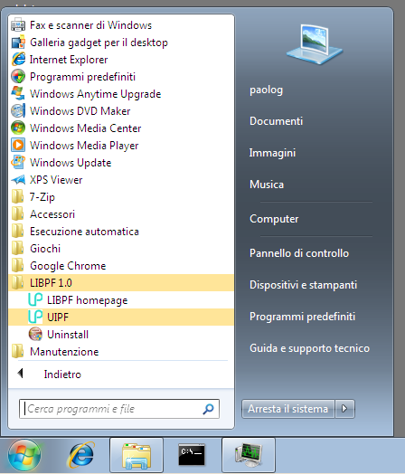
On Windows systems after installation, the user interface of LIBPF® is installed in Programs → LIBPF® 1.1. To launch the user interface, click on UIPF:
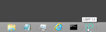
For your convenience, it is better to perform a right mouse button click on the application and select Add to the application bar in the lower menu, in this way whenever you want to start the LIBPF® user interface you will find the shortcut in the Desktop application toolbar:
On Linux systems the user interface of LIBPF® is available as an executable file /usr/bin/UIPF. It is possible to move the UIPF file in any favorite position (desktop, other folder, …) and run it: all data, results and settings are always stored in the kernel cache directory (/var/cache/LIBPF_1.1).
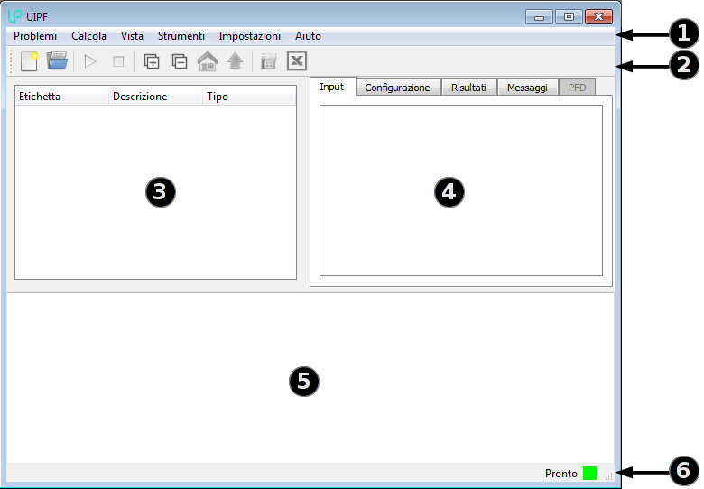
At launch, the interface looks like in the figure below, where you can identify the 6 main areas:
-
Menu bar;
-
Tool bar, which presents a selection of the most frequently used commands;
-
Tree view panel, which shows a structured view of various elements (streams, units, reactions) that make up the process;
-
Details view panel, where you can examine the input and results, and display the connectivity for the flowsheets.
-
Message panel, where diagnostic messages from the calculation engine are shown;
-
Status bar, where confirmation messages appear and where a small box (green in the figure) is shown at the right side, and which becomes red in case of errors.
Case management
Unlike most tools for process simulation, the LIBPF® user interface does not use files to save the results of the simulations, but relies on a database.
This is possible because the interface does not allow the user to change the configuration of the process, but only the operating parameters and options that have been made available by the developer of the model. The distinction between configuration (fixed for all the simulations of a process) and operating conditions (which differ from one case to another) is analogous to the distinction between classes and the instance of an object in object-oriented programming and is a hallmark of the LIBPF® technology.
The difference between the conventional approach and the object-oriented one of LIBPF® is illustrated in the following two tables:
Conventional Approach
| General purpose program | Configuration / Operating conditions |
|---|---|
| Microsoft Excel | Model of process A in conditions 1 (fileA1.xls) |
Model of process A in conditions 2 (fileA2.xls) |
|
Model of process B in conditions 3 (fileA3.xls) |
|
Model of process B in conditions 4 (fileA4.xls) |
Object Oriented Approach of LIBPF®
| Special purpose program / Configuration | Operating conditions |
|---|---|
| LIBPF® application for process A | Conditions 1: case A1 |
| Conditions 2: case A2 | |
| LIBPF® application for process B | Conditions 3: case B3 |
| Conditions 4: case B4 |
The advantages of the object-oriented approach are:
-
Reduces the duplication of information;
-
Reduces the possibility of making errors (e.g. a comparison of process A in conditions 1 and 2 requires that the Microsoft Excel files
fileA1.xlsandfileA2.xlsdiffer only on the operating conditions, and not on the calculation details of the model – but it is easy to make mistakes!); -
Allows you to systematically update a series of scenarios (a set of cases) with a new version of the process (e.g. with more accurate models).
In a typical installation on Microsoft Windows the used database has Access format (although it is not required that Microsoft Access be installed) and is located in the }persistency.mdb file in the working folder within the current user profile, typically in C:\ProgramData\LIBPF 1.0.
Creating a new case
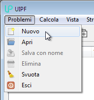
You can create a new case in the LIBPF® user interface with the Case → New command from the menu bar:
or with the corresponding button in the toolbar:

The program shows a dialog box which allows you to choose the process configuration (typically a single LIBPF® application can manage various configurations), and give a name and description to the case:
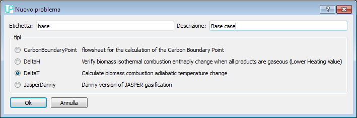
There are limitations regarding the allowed characters in the name and description fields:
-
The first character of the description must be alphabetic, while the subsequent characters may be alphanumeric, space or any of the following characters:
,:-_{}<>[]. -
The first character of the name must be alphabetic, while the subsequent characters may be alphanumeric, space or any of the following characters:
,-_{}<>thus compared to the description, the:[]characters are specifically excluded. -
By alphabetic character the characters in the
a – zandA – Zrange are intended (case sensitive), along with all the accented characters (àáâãäåèé...) and generally all the characters considered alphabetic in the main languages (i.e.α – ω,Α - Ω,А - Я,а – я…); -
By alphanumeric character an alphabetic character or a digit (
0 – 9) is intended.
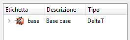
When the user gives the confirmation, the interface starts the computing kernel which instantiates an object of the chosen type (DeltaT in this case) with the name (“base” in this case) and the description (“Base case” in this case) provided by the user, saves it in the database and then opens it. Note that results are not available as no calculation has been performed yet.
At the end of these operations the LIBPF® user interface is ready for changing the inputs and launching the calculation, see the related chapters Editing input data and Calculation).
Saving a case with a new name / description
After examining the results, you can decide to create a new case by starting with the current one, with respect to which you may wish to change some operating conditions.
For example if the current case is the “Base case” case, you might want to create a new “75 percent case” case to calculate the operating conditions at reduced load. To do this, use the Cases → Save as command:
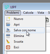
which duplicates the current case in the database, applying the provided description:
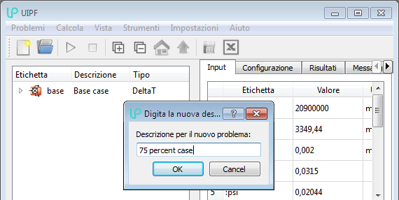
For the characters accepted in the description field, the limitations specified at the Creating a new case chapter apply; a description like “75% case” is not accepted because the % character is not allowed.
Beware: the new case is not immediately loaded in the interface: you must explicitly retrieve the new case, in the manner described in the next chapter Retrieving an existing case.
As more fully explained in the Editing input data chapter, any modification of the operating conditions via the graphical interface is immediately applied to the current case. This is why it is important to use the Save as command and then immediately load the new case before you start editing anything, otherwise you’ll be modifying the current case!
Retrieving an existing case
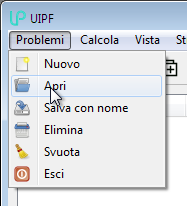
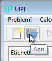
As you proceed with the work, all the generated cases are saved in the database. At any time you can re-open a previously created case with the Cases → Open command:
or with the corresponding button on the toolbar:
The program will then display a list of the existing cases, from which you can choose the one of interest:
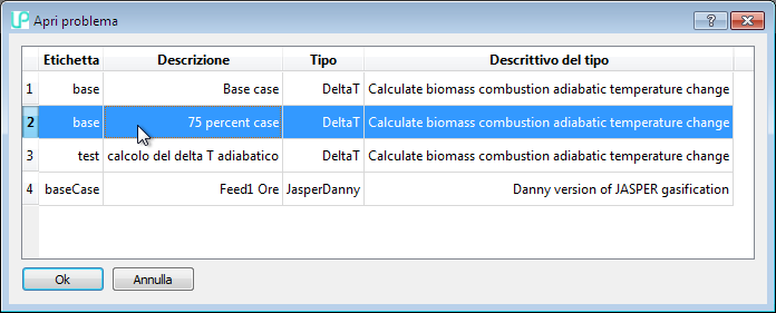
Beware: after loading the case the calculation isn’t launched: the cases are saved in the database immediately after being calculated, thus the graphical interface can restore the complete state (input and results).
Removing an existing case
If for any reason the current case is no longer of interest, you can delete it from the database with the Cases → Delete command:
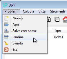
Note: the command is available only after having loaded the case.
Nota bene: the deletion of a case is an irreversible process, and does not require confirmation: proceed with caution!
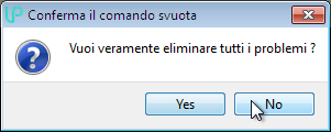
Also, if there are too many cases in the database, or you want to reset the work done, you can clear the database completely. For this purpose you can use the Cases → Empty command:
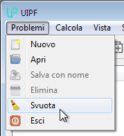
Nota bene: emptying the database completely is an irreversible process and with extensive consequences (e.g. it also deletes cases generated with another LIBPF® application that are saved in the database, even if they are invisible from the interface), this is why an explicit confirmation is required:
It is advisable, in case of doubt, to create a copy of the database (persistency.mdb located in the above mentioned location) manually (copy-paste of the file) in a safe location (i.e. Documents\backupDataBases).
Organization of objects and sub-objects
When a case is opened with the interface, a structured view of various elements (streams, units, reactions) that make up the process is displayed in the tree view panel.
The program uses various icons to indicate the type of object:
| Icon | Description |
|---|---|
 |
flowsheets and sub-flowsheets |
 |
the folder containing all the streams |
 |
the folder containing all the units |
 |
a material stream |
 |
a phase (normally contained in a stream) |
 |
a unit (e.g. a compressor or a reactor) |
 |
a chemical reaction |
 |
a multi-reaction (a particular type of reaction that shifts the species from one stream to another, used in the membrane and fuel cell unit) |
 |
unknown object (this icon should never appear) |
Just after opening a case, the root element (the one at the top) represents the current case. You can navigate through the objects and sub-objects by double-clicking (single clicking on linux systems) on the line in the tree view, which changes the selected object: as you enter the tree structure, it only shows more objects contained in the current object.
For example starting with this kind of view:
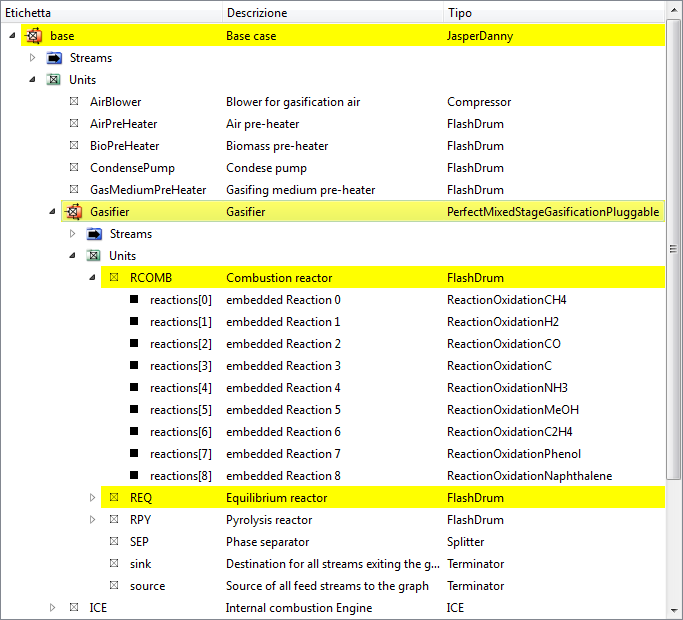
by double-clicking on the Gasifier the view will change this way:
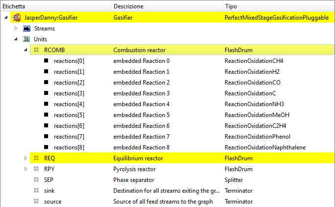
note the full path to the object: JasperDanny:Gasifier; in the full paths towards the variables the colon character is used (:) to separate objects from the sub-objects, and period (.) to separate the object from the variable.
Continuing the examination of the sub-objects contained by the Gasifier, by double-clicking on RCOMB the tree view will become:
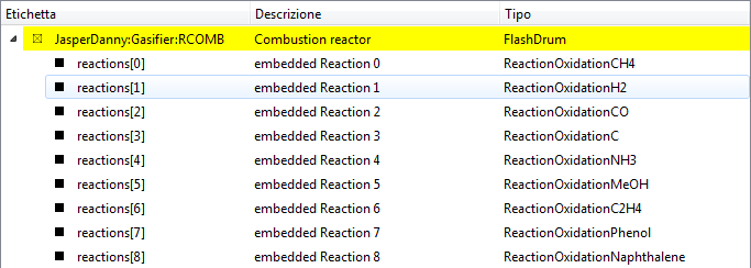
and lastly by double clicking on reactions[1] only the current object will be shown (as the reaction does not contain sub-objects):
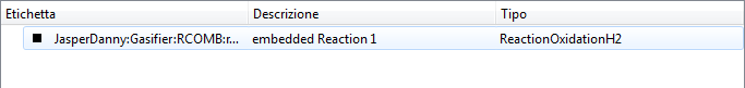
note the full path to the object: JasperDanny:Gasifier:RCOMB:reactions[1]; for the vectorial objects or variables the square brackets [] suffix operator selects the object of interest with an integer index starting from zero, for example reactions[0] is the first reaction and x[5] is the sixth mole fraction.
The Stream folder contains Stream-type objects each with the thermodynamical state (T, P) and the Phases as sub-objects, both the separate phases that compose the material and the total phase (if there is more than one phase). The Units folder contains sub-flowsheets and unit operations, each with its operating specifications and key performance data (deltaP, duty, deltaH, deltaS, efficiencies, …). Unit operations can also contain the reactions with their stoichiometric coefficients, equilibrium constants and rate of conversion.
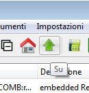
To go in the structure up with a single level, you can use the View → Up command from the menu bar:
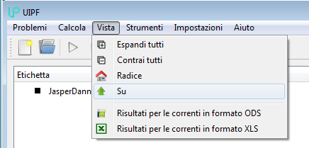
or the corresponding button in the toolbar:
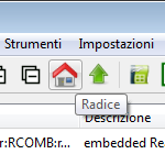
To go up again to the highest level in the structure you can use the View → Root command in the menu bar:
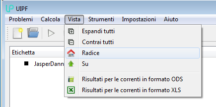
or the corresponding button in the toolbar:
Once the object of interest selected, you can examine the details in the panel at the right (details view) which has four tabs:
-
Input: user-specified parameters, read-write
-
Results: selection of key results, read-only
-
Messages: warnings and errors, read-only
-
and PFD (Process Flow Diagram), clickable.
The last tab is active only for flowsheets and sub-flowsheets, and allows to see their process scheme and zoom in or out, and to examine the sub-objects by interactively clicking on the units or streams in the PFD view: the effect is equivalent to a double click on the corresponding object in the tree view on the left.
Simulation
Editing input data
The user interface allows you to set the operating parameters and conditions and change the options that have been made available by the developer of the model. This implies that some input parameters could be inaccessible, because the developer of the model considered them unattractive or even dangerous to handle (e.g. for the stability, accuracy and convergence of the model).
With these limitations, editing is very straightforward: just browse the tree view and identify the stream, unit, sub-flowsheet or reaction you want to edit, and double-click. For example if you want to change an input parameter relative to the reaction[0] reaction of BiomassReaction_pyro_max type in the RPY unit of FlashDrum type found in the Gasifier sub-flowsheet of PerfectMixedStageGasificationPluggable type, just browse the tree view and double click on the Gasifier:RPY:reactions[0] object:
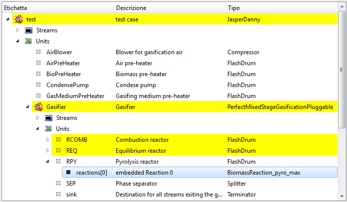
so that you change the tree view, which shows now the current object:

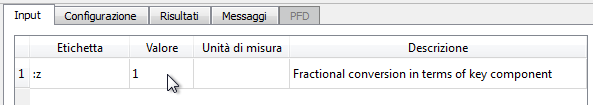
The details view panel now shows a filtered view of the details relative to the selected reaction; particularly clicking on the Input tab the input variables that can be manipulated (only one in this case, the conversion) are shown:
At this point just click in the box and type in the new value:
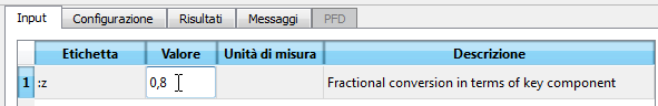
The change becomes effective after you press Enter or click on another element in the user interface (i.e. removing the focus from the input field).
Any change made to the operating conditions carried out this way via the graphical interface is immediately updated in the database with reference to the current case. For this reason explicitly saving the changes as we are used to do in other programs isn’t necessary: the Cases → Save does not even exist, there is instead Cases → Save as, which is used to create a copy of the current case (see the Saving a case with a new name / description related chapter).
Calculation
When a new case is created, results are not available as no calculation has been performed yet (see Creating a new case). Also if an existing case is loaded (see Retrieving an existing case) or the current case is edited (see precedent chapter Editing input data), you need to explicitly launch the calculation.
This logic is advantageous if the simulation runs are of considerable duration: if the calculation started automatically after each change, this could render the graphical interface interface unresponsive.
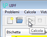
In any case you can launch the calculation of the current case with the Calculate → Calculate command:
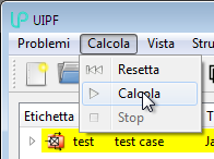
or with the corresponding button in the toolbar:
The calculation is delegated from the graphical interface to an executable, the calculation kernel, which is launched as a separated process, as you can see from the notice indicated in the status bar at the bottom right.

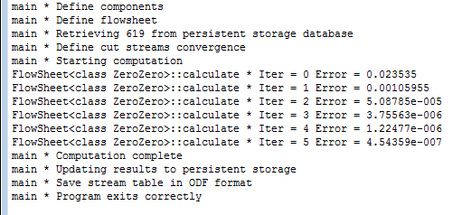
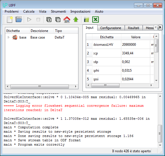
During the calculation in the bottom panel (of the messages) the diagnostic messages coming from the kernel are shown in real time, in order to monitor the progress of the calculation. A typical trace in case of success would be:
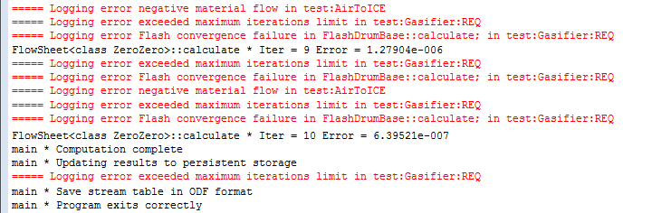
If instead during the calculation errors occur, these are highlighted in red in the messages panel:
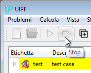
In these anomalous situations the duration of the calculation could go on for too long, and seen the encountered errors the results will certainly be devoid of interest; if needed in these cases you can stop the calculation using the Calculate → Stop command:
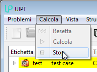
or with the corresponding button in the toolbar:
At the end of every calculation you can examine the results in the manner specified in chapter Examining the results.
Homotopy
Homotopy is a globally convergent numerical continuation method for solving systems of non-linear equations. With homotopy, to solve a complex problem, you solve first a simpler problem and then continuously transform it so that its solution is transformed into the solution of the complex problem. During this transformation it is possible to track what happens to the equations and to the solution, so that the speed of the deformation can be adapted.
Within the LIBPF® User Interface it is possible to to solve in homotopy mode:
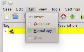
This solution mode is useful when the process is very sensitive to changes to certain input parameters, or when the desired step change for those parameters is relatively large. In Homotopy mode all the input variables whose values have been changed by the user since the last computation are moved simultaneously and gradually from the previous state to the new desired state, repeatedly solving the model for the intermediate values.
Examining the results
Calculation status
At the end of a calculation or even after having created a new case the user interface will display something similar to this figure:
Firstly note in the status bar at the bottom right the “Node 426 has been opened” notification: this number is internally used by the database to uniquely identify the current case.
In the top left panel (tree view) the program uses color codes to indicate at a glance the status of the last calculation:
-
white indicates: no error nor warnings:
-
yellow indicates: there are warnings:
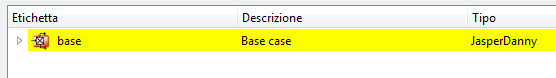
-
red indicates: there are errors:
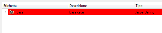
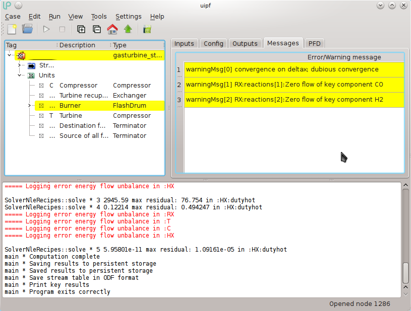
In case of warnings or errors the color codes are displayed on each object to make the search for the cause easier:
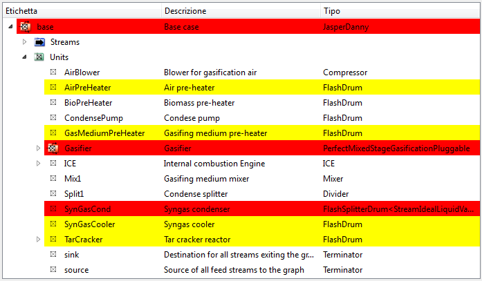
From this example you can see that the (“base”) case contains errors (red line) because the Gasifier and SynGasCond sub-objects contain errors. The AirPreHeater, GasMediumPreHeater, SynGasCooler and TarCracker contain warnings (yellow lines), but the errors prevail in determining the global state of the case.
Details and descriptions about the errors and warnings can be found in the Messages tab for each unit, with the same color conventions of yellow for warnings and red for errors:
Results
You can find the results for various units and streams in the “Results” tabs from the panel at the right (details view) by browsing through the objects and sub-objects as shown in the Organization of objects and sub-objects chapter.
These tables allow selecting a subset of cells or the entire table, and copying that to the clipboard:
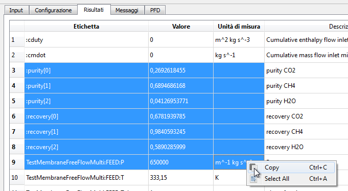
For the selection in the screen-shot, the text copied to the clipboard will include the column header and the content of the selected cells, with tabs (character ⇥) as separators of the fields:
Tag ⇥Value ⇥Units
:purity[0] ⇥0,269262 ⇥
:purity[1] ⇥0,689469 ⇥
:purity[2] ⇥0,0412695 ⇥
:recovery[0] ⇥0,678194 ⇥
:recovery[1] ⇥0,984059 ⇥
:recovery[2] ⇥0,589029 ⇥
TestMembraneFreeFlowMulti:FEED:P ⇥650.000 ⇥m^-1 kg s^-2
The content of the clipboard can then be directly pasted to a spreadsheet, and the tabs will be interpreted as column separators.
The results for the material streams (material and energy balances) can be exported to a spreadsheeting program such as Microsoft Excel (if available) on the supported Microsoft Windows operating systems, or LibreOffice (if available) on all supported operating systems, as shown in the following two paragraphs.
Concerning numerical values, the LIBPF® user interface uses the global system settings for the number formats (comma or dot as decimal separator etc.).
Units of measurement (UOM)
The LIBPF® user interface currently supports three sets of units of measurements: SI (International System of Units), EN (imperial units) e Eng (engineering units). The default settings is SI, which is also the unit sets internally used by the kernel for all the computations. It is possible to change the units of measurements for all the variables by selecting the menu Settings → Units:
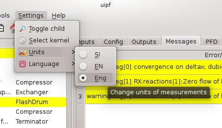
Whenever the global unit setting is changed, all inputs and results are presented in the selected units from that moment on, and the previously set values are converted so that results must actually be unchanged.
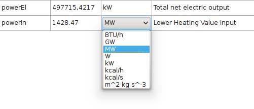
Besides these global units of measurements settings, the LIBPF® user interface also supports setting units for each individual variable, both in input and in output forms. These settings can be changed by pulling down the combo boxes “Units of measurements" found to the right of each variable. As soon as the unit is changed, values are automatically converted.
The supported units of measurements are listed in this table, grouped by the underlying physical quantity.
Exporting material and energy balances to LibreOffice
If a program that can open the OpenDocument ODF format such as LibreOffice has been installed, you can export all the material and energy balances for the material streams table by using the View → Results for streams in ODS format command:
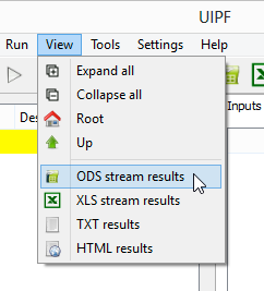
or with the corresponding button in the toolbar:
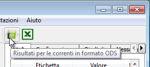
Note: the command is available only after having carried out the calculation.
Also in this case, the spreadsheet will open in a few seconds:
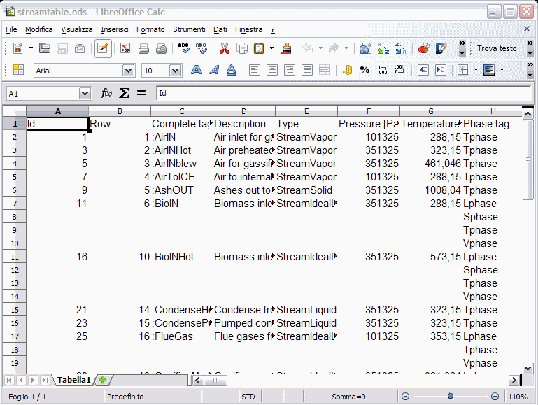
The operating logic of this command is very different of the one described in the following chapter Exporting material and energy balances to Microsoft Excel; in this case no macro is run in LibreOffice, but rather the streamtable.ods file is directly generated starting from certain files produced by the calculation kernel (particularly content.xml, which is produced at the end of each calculation). This implies that the streamtable.ods file is rewritten each time, thus you can’t keep a “formatted” sheet that presents the same results properly formatted, as in Microsoft Excel. In addition due to the inner workings of LIBPF®, the data for each stream and each phase is arranged by row instead of column as in the case of Microsoft Excel, which makes reading difficult.
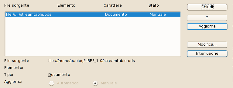
The approach to create a readable format is to create an independent LibreOffice file e.g. formatted.ods and take the fields of interest by creating a link between the formatted.ods and streamtable.ods files, for example:
=file:///home/paolog/LIBPF_1.0/streamtable.ods’#$Tabella1.$A$1
The LibreOffice INDEX(reference, row, column) function may be useful, as it allows you to switch from a row view to a column view.
By creating such connections, the formatted.ods file will remain permanently linked with the streamtable.ods file; at each new run you will be able to update the formatted.ods file in four steps:
-
Using the View → Results for streams in ODS format command in the LIBPF® user interface;
-
Closing the this way rebuilt
streamtable.odsfile which will open automatically (examining or editing this file is not of interest); -
Using the Edit → Links command for
formatted.odsin LibreOffice: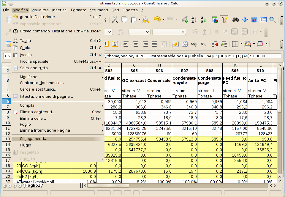
-
Clicking on the “Update” button and closing the dialog box:
Exporting material and energy balances to Microsoft Excel
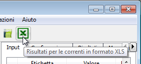
On supported Microsoft Windows operating systems, if the Microsoft Excel is installed, you can export all the material and energy balances for the material streams table by means of the View → Results for streams in XLS format command:
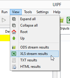
or with the corresponding button in the toolbar:
This command opens the streamtable.xls file in Microsoft Excel, and launches a macro written in Visual Basic for Applications which reads the needed values from the Microsoft Access database loading them in the “rawdata” sheet of the file.
The “formatted” sheet presents the same results properly formatted:
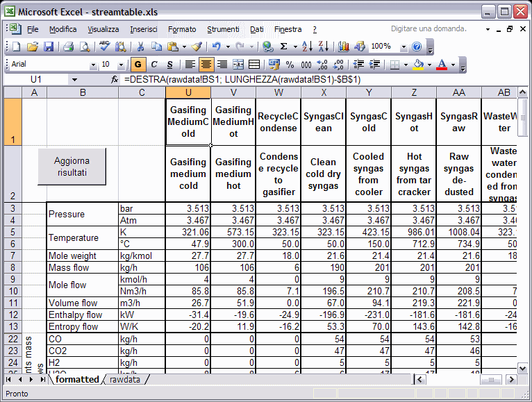
Beware to the displayed columns in the formatted sheet: it may be necessary to extend or reduce the number of those columns appropriately to handle flowsheet with more or less streams. If it is necessary to increase the number of formatted columns, select the last column to the right then click on the fill icon in the top-right corner then pull to the right; after that, remove the columns which display no stream name.
You can leave the Microsoft Excel window open and press the “Update results” button to re-run at any time (e.g. after a new calculation) the macro: this file will keep pointing to the object that was open in the LIBPF® user interface at the moment when the command of opening Excel has been given.
Exporting all data to a text file
It is possible to export all the data for the currently open object and all its sub-objects, saving them to a text file (.txt). This functionality is available in the “View” menu by clicking on “TXT results”:
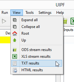
When this command is clicked, the current model (more precisely the node currently open in the tree view) is exported to a plain text file named ID.txt where ID is the model identifier in the database. The generated text file is automatically opened and displayed in the Operating System default application for opening text files (i.e. Notepad).
Exporting all data as XHTML
It is possible to export all the data for the currently open object and all its sub-objects, saving them in HTML format. This functionality is available in the “View” menu by clicking on “HTML results”:
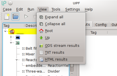
When this command is clicked, the current model (more precisely the node currently open in the tree view) is exported to a number of separate XML files, which are placed in a temporary directory together with a dozen auxiliary files.
The XHTML file named index.xhtml is automatically opened by the Operating System default application for opening HTML files (which must be one of the supported browsers), and from there it is possible to browse all sub-objects by following the links.
Sensitivity analysis
Very often in the course of a project sensitivity studies need to be performed. These sensitivity studies are very repetitive and only consist in changing one or more parameters (controlled variables) in a certain range for a certain number of points, by running a simulation for every point and recording in a table a certain number of results (monitored variables).
To automatize these tasks the LIBPF® user interface has a multi-dimensional sensitivity analysis feature. In practice this tool allows you to determine how sensitive a model is to the variation of the values of the parameters and assess how will the variation of the value influence the behavior of the model; it also provides assistance for the selection of the so-called “critical” variables, that is those whose deviation from the nominal value influences the performance indicators the most; with this tool you can acquire a lot of information about the model and the process in a short time.
The sensitivity analysis tool of the LIBPF® User Interface allows you to carry out several simulations by controlling one or more variables while maintaining all the other unchanged, and monitoring the effect on one or more results.
If you click on Tools → Sensitivity analysis:
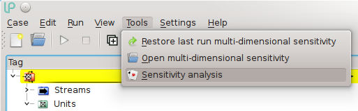
a window will appear with three tabs: “Control”, Monitor and Results:
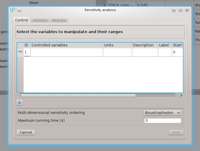
On the Control tab it is possible to select one or more controlled variables (at least one is required), setting the units of measurement, the optional label to display in the results table ad column header, the start and end values for the range to scan and the number of points the range must be divided into. The table comes pre-filled with one row, it is possible to add additional controlled variables by clicking on the “+” at the bottom left. It is possible to remove a previously set controlled variable by clicking on the “-” button on the left side of each row.
In the lower part of the window it is possible to set the sensitivity execution order (natural, the default boustrophedon or quasi-spiral) and the maximum running time. The sensitivity execution order is important if there are some regions of the scanned domain where convergence is difficult. The maximum running time, if set to a value strictly greater than zero, is interpreted as a time-out expressed in seconds - if the sensitivity runs for so long, the run is interrupted and the results collected up to that point will be displayed.
The user can choose the controlled variable from the list of all the variables that can be specified for the current case (these are the variables that appear in the “Input” tab of the units and streams).
As soon as one controlled variable has been chosen, or its selection has been changed, the program updates the units of measurement and initializes the start and end sensitivity limits with the current value of the variable; the description of the variable is also shown. The user must typically only change one of the two limits and probably set the number of points to a value greater than the default value equal to 1 that would reduce the sensitivity to the execution of a single run.
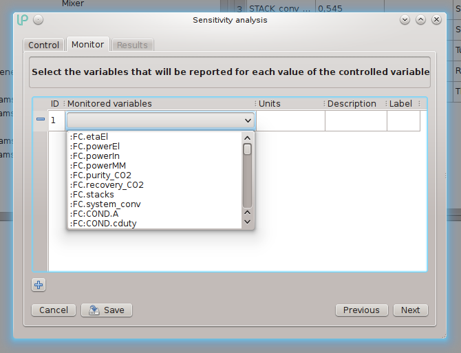
At this point you can press “Next” to proceed to the “Monitor” tab where you can choose the variables (results) to be monitored.
The user can choose the monitored variables from the list of all the results for the current case. As soon as a variable has been chosen, or its selection has been changed, the program updates the units of measurement, the description and the label of the variable. If desired, the user can change the label, which will be shown as a header in the corresponding column of the results table.
The table of monitored variables has a variable number of rows, however, greater than or equal to one (it does not make sense to follow a sensitivity study without monitoring at least one variable). The user can add new rows or remove the existing ones by using the plus (+) and minus (-) buttons.
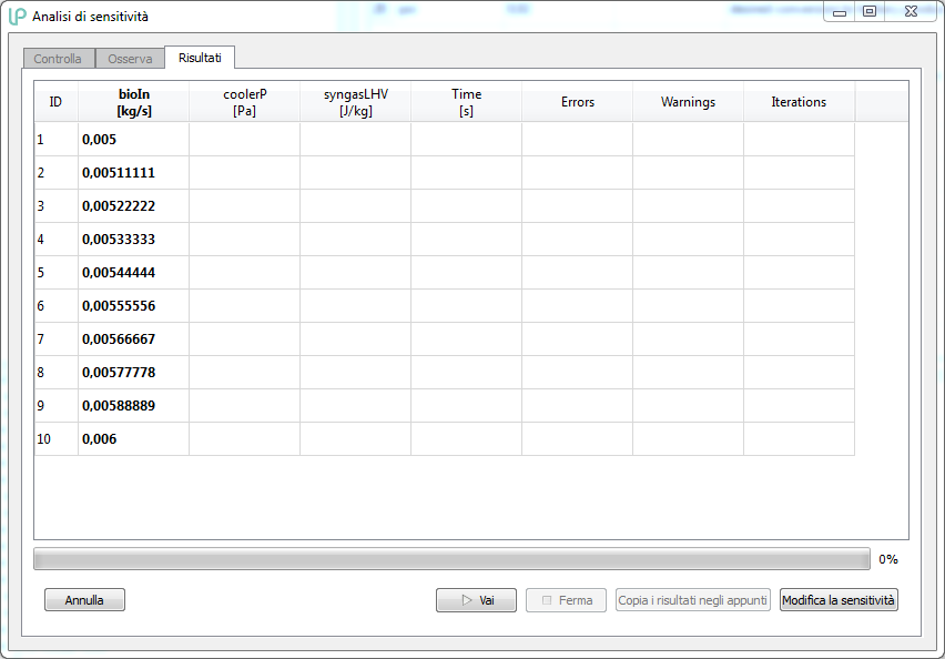
At this point you can click “Next” to proceed to the “Results” tab from which you can start the sensitivity analysis by clicking on the “Go” button; before doing so, form this dialog you can also save the configuration of the current sensitivity analysis by clicking on Save (see below, Saving and loading sensitivity analyses).
Note that once arrived at the “Results” tab the two previous tabs are frozen, i.e. the settings for the controlled variable and for the monitored variables can no longer be changed. In fact, the “Edit sensitivity” button functions as a “back” button: unlocks the “Control” and “Monitor” tabs and allows you to change any settings.
If instead a sensitivity analysis is launched, the LIBPF® user interface starts the calculation kernel. During the execution the rows relative to each value of the controlled variable are highlighted while gradually proceeding to the calculation, and the results of the monitored variables are tabulated as soon as they become available. You can at any moment copy the table (by pressing the “Copy results to clipboard” button), stop (by pressing the “Stop” button) and resume (by pressing the “Go” button) the execution of the calculation.
The rows are color coded highlighted according to this table:
| Grey |  |
Row in execution |
| Green |  |
Row executed without warnings or errors. |
| Yellow |  |
Row executed with warnings |
| Red |  |
Row executed with errors (results are available, but probably not valid) |
| Dark Red |  |
Row not executed because of a serious internal error of LIBPF® (no results available) |
| Purple |  |
Row not executed because of a LIBPF® crash (no result available) |
| Dark cyan |  |
The row is not completely executed because of an user break (no results available) |
The table generated in this way can be copied to the clipboard (by pressing the “Copy results to clipboard”) and from there into a spreadsheet.
Note: at the end of the sensitivity the interface substitutes the value assumed by the controlled variable in the last run in the appropriate Input box so that the loaded case results amended.
Saving and loading sensitivity analyses
If you click on the Save button on the Monitor tab once you have fully specified your sensitivity analysis, a small modal dialog appears:
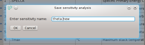
where it is possible to enter a meaningful name for the sensitivity, up to 50 characters long, containing any character except the following reserved characters: < (less than) > (greater than) . (period) : (colon) " (double quote) / (forward slash) \ (backslash) | (vertical bar or pipe) ? (question mark) * (asterisk) _ (underscore) , characters whose ASCII integer representations are in the range from 0 through 31 and $ (dollar sign).
If the supplied name has already been used to save a sensitivity for the current type, the user is asked for overwrite confirmation, else the sensitivity is saved to an XML file in the working folder, with a full name that contains both the sensitivity name and the current type name.
Saved sensitivity analyses can be loaded back using the Open multi-dimensional sensitivity dialog box that is available under the Tools menu:
The following dialog box appears:
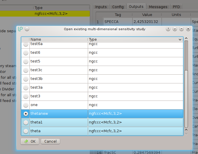
The dialog shows the list of available saved sensitivities along with their model types; the saved sensitivities whose type is equal to the type of the currently loaded case are highlighted in light blue. Typically it makes sense to retrieve a previously saved sensitivity for the same type as the current type, but advanced users can exploit the power of loading an existing sensitivity for a similar type, provided they know how to adapt it if required.
Settings
From the settings menu you can change some of the general settings of the application:
-
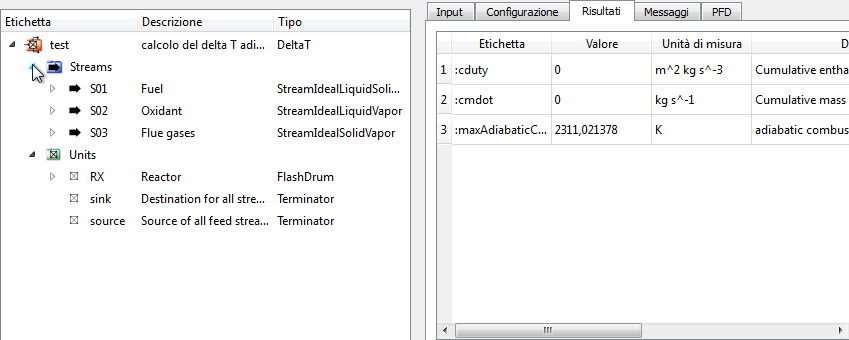
Toggle child: toggles the viewing in the details view panel of the input variables and of the results of the objects in the currently selected object in the tree view; for example if the currently selected object is the deltaT flowsheet, and the viewing of the “children” is disabled, the interface could look like this:
if instead the viewing of “children” is activated, the interface could look like this:
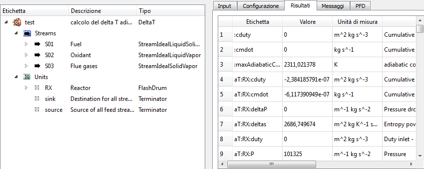
note how in the details view panel the results of the internal objects of the flowsheet have appeared, recognizable because the label contains the complete path to them (e.g. RX:P is the pressure of the RX unit);
-
Select kernel: if more calculation kernels have been installed (each of which can simulate various components and processes) this command allows you to switch from one kernel to another;
-
Units: to choose the units of measurements for the display of physical quantities;
-
Activate: allows you to start the automatic activation procedure (see the LIBPF® Activation Guide);
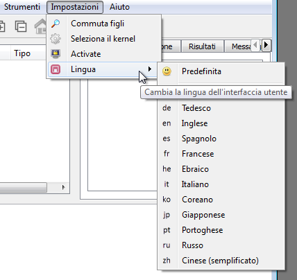
-
Language selection: from here you can change the language of the user interface (the default is set to the language of the operating system); note: the language selection is only effective after restarting the LIBPF® user interface.