Heterogeneous equilibrium reactions

[It’s time for a chemeng-related post on the blog, which has drifted in the technicalities a bit in the past few months …]

Unit operation models and process flowsheets in a simultaneous formulation result in systems of algebraic equations (NLAE = Non Linear Algebraic Equations). The chemical and phase equilibria can be formulated as a minimization problems, but in the framework of integrating these equations with process flowsheeting, that is not practical.

For these reasons in LIBPF the simultaneous phase and chemical equilibrium in reactive flashes, and the simultaneous phase equilibrium, chemical equilibrium and heat transport rate laws in reactive exchangers are handled in general using the algebraic formulation of the equilibria.

For each reaction equilibrium an additional equation is created, to equate the thermodynamic equilibrium constant K, function of temperature only, and K_ist, the current value of the equilibrium constant (from German “ist-Wert” = current value), function of the fugacities of the components. The corresponding additional unknown is the rate of reaction, typically expressed in kmol/s.

If the chemical equilibrium is heavily shifted in one direction (either maximum conversion with complete exhaustion of one or more reactants, or zero rate of reaction) then numerical problems can arise in the solution of the associated algebraic system of equations. These  challenges are met in LIBPF by adding “intelligence” in the functions calculating the residuals, and by proper scaling of the unknowns; in this way, all effort goes into the formulation of the problem and no customization of the solver is required.

Recently the peculiar challenges related to heterogeneous reactions have been addressed. The remarkable difference w.r.t. homogeneous equilibrium reactions is that in the heterogeneous case as soon as the second phase disappears, the equilibrium does not hold anymore, and the K can and should be different from the K_ist.

For example, if table salt (NaCl) is present as a solid in equilibrium with its solution in water, the product of the ion activities must be equal to the equilibrium constant; but if the solution is not saturated, and there is no solid at all, then the product of the ion activities will be lower than the equilibrium constant: K_ist < K.

Another example is the Boudouard reaction:

2·CO  ⇄ C(s) + CO₂

When all species are present, the carbon black decomposes or is formed in a way to keep constant and equal to K the value of K_ist. For a gas phase only composed by CO and CO₂ there are three species present, but only one concentration can be imposed: the other two derive from the mass balance and from the equilibrium.
When the solid phase disappears (and this happens at temperatures higher than about 700 °C, when carbon monoxide is stable), there are two species present, and as before only one concentration can be imposed: the other derives from the mass balance. The value of K_ist, can now assume any value, provided it is higher than the equilibrium constant: K_ist > K (note the reversal of the direction of the disequality, because here the solid is a reaction product).

But enough theory, let’s see some code and some nice pictures.

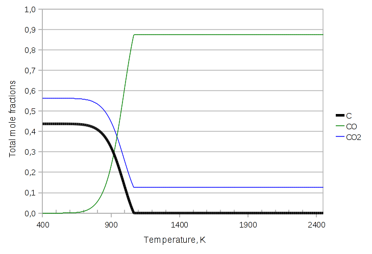
First here is the code to calculate the composition of the equilibrium when only C, CO and CO₂ are assumed present, for an equimolar feed mixture:

// define components
components.addcomp(new purecomps::carbon);
components.addcomp(new purecomps::CO);
components.addcomp(new purecomps::CO2);
// instantiate and initialize streams
StreamIdealSolidVapor feed(-1); 
feed.Tphase->calculateX(MassBalanceMode::N);
StreamIdealSolidVapor product(-1);
// instantiate the reactor
std::list<std::string> r = boost::assign::list_of("ReactionBoudouardEquilibrium");
FlashDrum reactor(r);
// connect
std::string in("in");
reactor.attach(feed.id(), in);
std::string out("out");
reactor.attach(product.id(), out);
// generate table
std::cout << "T\tC\tCO\tCO2" << std::endl;
for (feed.T = Tmin; feed.T < Tmax; feed.T += Tincr) {
  // initialize variables
  reactor.T = feed.T;
  // calculate
  feed.calculate();
  reactor.calculate();
  // print selected results
  std::cout << feed.T << "\t" << product.Tphase->frac() << "\t" << product.Tphase->frac(1) << "\t" << product.Tphase->frac(2) << std::endl;
} // iterate over T

The results are:

Here CO2 is invisible because it is behind the thicker solid carbon C line. In this case the solid carbon becomes less and less at higher temperatures, but never quite disappears (which is apparent from the smooth, sigmoidal form of the curve).

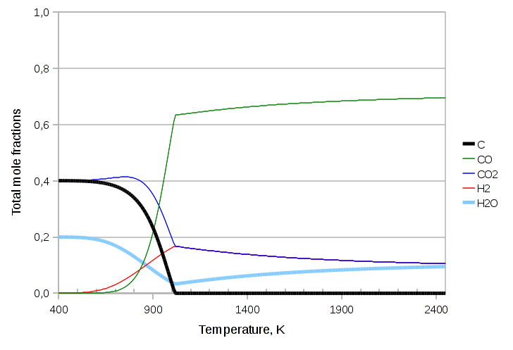
The next exercise makes visible the idiom “pushing the equilibrium”; here there is much less CO in the feed. In the code we just need to add the three lines after the feed stream is constucted:

feed.Tphase->Q("ndotcomps[CO2]")->set(4.0, "kmol/s");
feed.Tphase->Q("ndotcomps[C]")->set(3.0, "kmol/s");
feed.Tphase->Q("ndotcomps[CO]")->set(1.0, "kmol/s");

The graph changes dramatically:

Now the solid carbon disappears at about 1065 K, which is confirmed by the discontinuity in the derivative of the curve. The disappearance of a phase can be a literal catastrophe for the numerical implementation, because an equality turns into an inequality, which would require the equation / variable count to be updated, the jacobian to be rebuilt etc. etc. The current unreleased, alpha version of LIBPF can handle all this without convergence errors.

In the next exercise we’ll throw in some additional atom, namely hydrogen, in the form of water. We’ll need to also add biatomic hydrogen to the components and the Water Gas Shift equilibrium reaction:

CO₂ + H₂ ⇄ CO + H₂O

The code we need to change is:

components.addcomp(new purecomps::H2); 
components.addcomp(new purecomps::water);
StreamIdealSolidVapor feed(-1);
feed.setTag("FEED");
feed.setDescription("Reactants");
feed.Tphase->Q("ndotcomps[C]")->set(3.0, "kmol/s");
feed.Tphase->Q("ndotcomps[CO]")->set(1.0, "kmol/s");
feed.Tphase->Q("ndotcomps[CO2]")->set(4.0, "kmol/s");
feed.Tphase->Q("ndotcomps[H2]")->set(1.0, "kmol/s");
feed.Tphase->Q("ndotcomps[H2O]")->set(1.0, "kmol/s");
feed.Tphase->calculateX(MassBalanceMode::N);
StreamIdealSolidVapor product(-1);
product.setTag("PRODUCT");
product.setDescription("Educts");
std::list<std::string> r = boost::assign::list_of("ReactionBoudouardEquilibrium")("ReactionWaterGasShiftEquilibrium");

The resulting graph is:

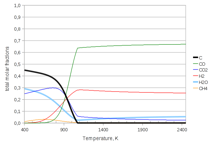
The last variant we’ll try is throwing in one last species: methane.

Code:

components.addcomp(new purecomps::methane);
//  . . .
feed.Tphase->Q("ndotcomps[CH4]")->set(1.0, "kmol/s");
std::list<std::string> r = boost::assign::list_of("ReactionBoudouardEquilibrium")("ReactionWaterGasShiftEquilibrium")("ReactionReformingEquilibriumCH4");

Graph:

One drawback of the algebraic formulation is that the model developer has to specify which reactions to include; in the Gibbs free energy minimization the reactions are implicit in the atom balances, and the modeler’s duty is limited to specifying the components.

But on the other hand, we know that the number of (linearly independent in the sense that the Brinckley matrix is not singular) reactions can never exceed the number of components minus one. So the algebraic formulation always results in less equations than the energy minimization formulation.

The decision which reactions to include is a matter of experience and sound judgement: in other words, you have to know in advance what type of results you expect from the model !